
Hydricity Blog
Initial Modeling
Table 1: Inputs for Analysis
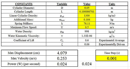
Figure 1: Calculations of Re, Sr and Fs

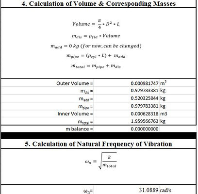
Figure 2: Calculation of Masses
Before the team was able to provide a complete numerical analysis of the prototype chosen for production, several modifications were made to the given model. The team was not necessarily certain that the chosen design would work as efficiently as possible, so the design conception and selection process was conducted an additional few times to ensure product operationality, durability, manufacturability and cost-efficiency. Therefore, the initial design chosen during Phase 1 was actually changed significantly by the team. The reason behind these notable design alterations stemmed from having a better understanding of the team’s problem statement during Phases 2 and 3, the desired outcomes and wants of the team’s advisors and the practicality of the manufacturing processes required for the alpha prototype.
The numerical analysis conducted by the team was extremely extensive, and it could not have been completed without a variety resources such as online engineering publications, experimental data from PhD theses, similar commercial product designs and even external advice and expertise from additional professors at Stevens. The team read, noted and analyzed around 10 engineering and research-based publications over the course of several weeks to try to make a more basic and understandable model without losing accuracy and credibility. In particular, the team based a majority of the modelling on vortex-induced vibration studies and the implementation of energy capturing devices. Like any engineering model, the team had to make several assumptions to achieve the desired outcome for various reasons. The team neglected any type of material defects, irregularities and surface roughness with the cylinder to make the fluid motion studies a bit easier to understand. Additionally, the team assumed that the fluid was invisicid, uniform and maintained a constant density (no external particles added to fluid). In real applications, the fluid can contain a mixture of dirt, sand, debris and even organisms. Lastly, the team assumed a constantly uniform and turbulent boundary layer. This is easily one of the most important assumptions, since the team was studying vortex-induced vibrations. Once the research was completed, the team consolidated these long pages of notes, formulas, assumptions and definitions into a usable engineering model.
After discussion with the team’s advisor, Excel was chosen as the primary program to conduct all numerical analysis. Excel was chosen for a multitude of reasons, mostly due to the accessibility of the program, as well as the team’s expertise in the various functions and features. MATLAB was also considered heavily, however, the team felt that this program could instead be used in the future to create a more appealing user interface such as an input and output result screens. The team decided to create a generic inputs table, seen directly below in Table 1, to better organize the data and to create a singular location where any input can be changed speedily and efficiently. Even though the formulas were not directly established by this point, the team decided that this was the best method of organization to keep the analysis concise, dynamic and accurate, and to not pollute the formula cells with long, confusing strings. The highlighted, yellow boxes indicate that these values are subject to change to understand the impact of each variable on the overall outcome of the device. This is extremely important because the team wants to maximize power output by adjusting these values accordingly and appropriately.
After establishing the desired constants for the setup of the numerical analysis, the team began constructing formulas within Excel one by one. Since the team is primarily dealing with fluid motion and vortex shedding, it was decided that the calculation of Reynold’s number should be conducted first to better understand the flow dynamics. Based on assumptions from Stevens’ fluid dynamics courses and online research, the team assumed that within a range of Reynold’s numbers from 300 to 300,000, the vortex profile the cylinder can be considered fully turbulent. Thus, strong and periodic vortex shedding will occur, which is exactly what the team desires. Next, the Strouhal number was calculated, which determines the vortex shedding frequency as a function of Reynold’s number. This calculation was used as an intermediate step to solve for the vortex shedding frequency. Above all else, this step in the analysis was easily one of the most critical calculations because this value must match the natural vibration frequency of the cylinder in order to create large amplitudes of cylinder displacement (amplitude directly correlates with power output). The calculation of Reynold’s number, Strouhal number and vortex shedding frequency is based on the above input values and is illustrated in Figure 1 below. These values will change as the inputs value change.
Once these three values were found, the natural frequency of vibration of the cylinder was the next calculation sought out for. This value needs to match the vortex shedding frequency so the cylinder in-flow will oscillate sinusoidally and within a range of desired amplitudes. However, another step must be taken before finding this value because the formula depends on the mass of the cylinder to determine the best spring constant to use (springs are located in shafts connected cylinders). To find the total mass, the mass of the pipe and the mass of the displaced water must be calculated. After assigning an appropriate spring stiffness value and calculating the total required mass, the natural frequency of vibration was found. This procedure is illustrated below in Figure 2.
With all of the values above calculated, the team was able to finally obtain the calculation of lift force, which was the final step in the pre-analysis phase. A lift coefficient of 0.6 was determined to be a conservative estimate based on extensive online research and previous experimentation. Therefore, the team assumed this value throughout the duration of the analysis. For the next sequence of analysis, the team had to do a bit of research and use Excel functions to plot the corresponding cylinder’s amplitudes, velocities and power outputs, since each function was dependent on time.