
Hydricity Blog
Induction Analysis
In the next step of the technical analysis, an analytical model of an induction system was made using Excel to realize the production of alternating current from the motion of the drivers in a 1 m/s current. This model allowed for the optimization of the induction system design, but prior to discussing the optimization, the theory and construction of the model will be touched upon. Ultimately, the team decided to analyze the design of an induction system rather than the rack and pinion to alternator set-up since the induction system can be modified. While they both would produce alternating current in a similar manner, the alternator set up would use a store bought alternator, which could not be altered to increase power output. Additionally, the induction system could generate electricity from non-uniform oscillatory motion of the drivers. A design that attempts to generate direct current with an alternator by converting the oscillatory motion of the drivers to a single rotational direction using a crank shaft would fail in the very likely case of non-uniform motion since the design would rely on motion with a particular steady amplitude. With that being said, the induction system was modeled in Excel using Faraday's Law as the central governing equation. This equation can be seen below:
As seen in the equation, the product of the number of loops in a coil (N) and the change in magnetic flux over the change in time (dΦ/dt) equals an induced emf or “voltage” (ε). Essentially, when a magnet moves through an electric coil, the strength of the magnetic field that interacts with the coil is changing. When an emf is generated by a change in magnetic flux according to Faraday's Law, the polarity of the induced emf is such that it produces a current whose magnetic field opposes the change which produces it. The induced magnetic field inside any loop of wire always acts to keep the magnetic flux in the loop constant. So as the drivers push a magnet up and down in a coil, an alternating current will be produced. To calculate the induced emf, an equation had to be used that would determine the change in the magnetic field strength in relation to the center of the coil. This equation can be seen below:
As seen in the equation the magnetic field strength of a cylinder magnet is dependent on the remanence field constant (Br), the radius of the magnet (R), the height of the magnet (D) and the distance away from the face of the magnet (z). With this equation, the team was able to input amplitude data of the driver as “z” to find the change in field strength in later steps. Next, to calculate the change in flux (dΦ), the change in magnetic field strength would be multiplied by the cross sectional area of the coil (A). This equation can be illustrated below:
Figure 8: Faraday's Law Diagrams
From these equations, the final voltage could be calculated by looking at the change from minimum to maximum flux and the time required to reach that point. Once the voltage was defined, equations were set up to find the resistance in the coil to ultimately calculate the power output. The equation for resistance can be seen below:
This equation consists of the resistivity of the wire (⍴) multiplied by the length of the wire (L) divided by the cross sectional area of the wire (A). With the resistance equation now defined, the team was able to calculate the final power output as seen in the equation below:
The next step after defining all equations and theory was to create the model and use optimization tools for the design process. Prior to setting up the optimization solver, a few assumptions had to be made. It was generally known that the power output could be increased with a greater number of turns of the coil, a stronger magnet, and multiple overlaid coils. With this being known, the team assumed that a very thin wire should be used since the number of turns would be limited by height constraints of the coil. For the analysis, the team used a standard gauge of 28 copper magnet wire, which is the thinnest standard wire. The team also assumed that the magnet being used would be made of neodymium, a material renowned for its magnetic strength, with a remanence strength of 1.45 T, which is one of the stronger but affordable types. The team also assumed that the model would analyze a system with one coil, since it is known that the more additional coils would just increase the power from an already optimized value. After these assumptions were made, there was enough information to carry out optimization.
To carry out the optimization, the parameters which could be manipulated were set as design variables. These variables included the radius of the magnet (Rm), the height of the magnet (H), the number of turns in the coil (N), and the radius of the coil (Rc). For the optimization to run properly, limits were set on certain variables that would allow the optimized design to meet the design criteria. A table giving a breakdown of these limits can be seen below.
Table 4: Induction Optimization Constraints
The limits set on the magnet dimensions were meant to keep the weight and size of the magnet down since portability is one of the main constraints. Additionally, these components would be in the top portion of the device, so space is very limited. The same goes for the coil dimensions, which could not be too long or wide due to space, especially since the team desired to overlap additional coils on the coil designed through Excel optimization. Next, the objective function was chosen to be maximized. The objective function here was the flux at the point where z = 0 which was known to be the moment for the largest possible flux value. After solving, the optimized design for a single coil induction system was found as seen in Table 5 below.
Table 5: Induction Optimization Results
The resultant power from this design comes out to be 1.1 W, which is low but was to be expected. By adding additional coils around the optimized single coil, the power output was increased. With these additional coils, the number of turns would remain constant, but the cross sectional area would increase with each additional coil. As a result the length of wire used would increase as well as the resistance. The iterations to show the increase in power output with the addition of coils can be seen in Table 6 and Figure 9 below.
So in conclusion, it can be seen that a total of 9 overlapping coils could ideally produce 12 W per induction system. Given that the team planned on designing each driver to have an induction system on each side and a total of two drivers in the device, the overall power output in this ideal scenario would be 48 W, which compared to the power input from the fluid is 95% efficient. While this sounds great, this analytical model assumes that the reactive motion of the drivers will be ideal harmonic motion and that there will be no losses from other areas such as friction and conversions between AC and DC. So moving forward, it has to be expected that the final power output will not be as efficient as calculated.


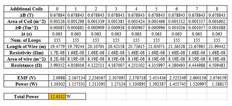

Table 6: Additional Coils
Figure 9: Power Output with
Additional Coils